How to Build FMECA and Fault Tree Analysis with MBSE

What Is FMEA?

FMEA is a proactive technique used to identify potential failure modes, their causes, and the effects of those failures on system performance. It involves analyzing the various components, subsystems, and processes of a system to anticipate and prevent failures.

FMEA helps identify and prioritize areas where improvements can be made to enhance reliability, safety, and maintainability. It uses a structured approach to evaluate the severity, occurrence, and detectability of potential failure modes, resulting in a risk priority number (RPN) that aids in prioritizing actions for mitigation.

What Is FMECA?

FMECA is a critical analysis required for ensuring viability of a system during operations and support phase of the lifecycle. A major part of FMECA is understanding the failure process and its impact on the operations of the system.

Figures 1 and 2 below show an example of how to model a process to include the potential of failure. Duration attributes, Input/Output, Cost and Resource entities can be added to this model and simulated to begin estimating metrics. You can use this with real data to understand the values of existing systems or derive the needs of the system (thresholds and objectives) by including this kind of analysis in the overall system modeling.

What Is Fault Tree Analysis?

Fault Tree Analysis (FTA) is a retrospective technique used to analyze the causes and consequences of a specific system failure or undesired event. It is primarily concerned with understanding the relationships between events that lead to a particular failure.

FTA starts with an undesired event, referred to as the "top event," and breaks it down into contributing factors using a logical tree structure. These contributing factors are represented as gates, which can be combined using logic operators (e.g., AND, OR) to model the causal relationships.

FTA helps identify the root causes and paths leading to the top event, facilitating the identification of critical points where mitigation measures can be implemented. In Figure 2, you can see how to use the Action Diagram to create a horizontal FTA. Using the action diagram for FTA allows us to not only identify the causes of failure and mitigate risks, but also calculate time, resources, and costs that could result in a system failure.

Figure 1. Vehicle Failure Process.

Figure 2. Failure Modes Expanded.

Step 1: Build the Model

Learn how to create Action Diagrams. Then use Figures 1 and 2 to develop your model.

Step 2: Add a Loop and Loop Probability

To enable the decision-making process regarding failure, you can create a loop that repeats at certain intervals. The timing of these decisions depends on two factors: the number of loop iterations and the duration of the "Continue Normal Operations" action.

To adjust the number of iterations:

1. Select the loop action labeled "Continue to operate vehicle?" (F.1)
2. Click the </>Script button (refer to Figure 3)
3. A dialog box will appear, allowing you to edit the action's script. From the pull-down menu, choose "Loop Iterations" and enter the desired number (as shown in Figure 4)

Figure 3. Vehicle Failure Process in Innoslate.

Figure 4. Loop Decision Point Script for 100 Iterations.

Next, modify the duration of the "Continue Normal Operations" actions (F.1 and F.4). Since the loop decision is not a significant factor in this model, you can assign it a small nominal time (e.g., 1 minute).

For the "Continue Normal Operations" action (F.4), select a duration of 100 hours. Combining this duration with a branch percentage of 90% for this path implies that there are approximately 900 operating hours between failures, which is typical for a vehicle in a suburban environment.

Note: You can provide a more precise estimate by incorporating a distribution for the normal operating hours.

Step 3: Add Decisions

The 90% branch probability comes from the script for the OR action (“F.2 Failure?”). That selection results in the dialog below.

Figure 5. OR Decision Point Probability Script Dialog.

For this example, assuming a failure occurs approximately 10% of the time, you can then determine whether the failure modes are probabilistic in nature or the paths need to be selected based on those probabilities. The second OR action (“F.3.1 Failure Mode?) shows three possible failure modes.

You can add more by selecting F.3.1 and using the “+Add Branch” button. You can use this to add more branches to represent other failure modes, such as “Driver failure,” “Hit obstacle,” “Guidance System Loss,” etc.

Note: Change the default names (Yes, No, Option) to the names of the failure modes, just click on the branch name and the name will appear on the sidebar, as in Figure 6. Just type in the name you prefer.

Figure 6. Changing the Branch Name.

Step 4: Add Time

To finish off this model add durations to the various other actions that may result from individual failures. The collective times represent the impact of the failure on the driver’s time. You can estimate using Triangular distributions of time (see sidebar in Figure 7).

Figure 7. Adding Time to the Action.

This shows an estimate from a minimum of ½ hour to a maximum of 1 hour, with the mean being ¾ hour. If you do this for the other actions, you can now execute the model to determine the impacts on time.

Step 5: Add THE Cost

1. Create an overall cost entity, such as "Failure Costs."
2. Break down the overall cost entity into various costs associated with repairs.
3. Assign the costs to specific actions using a Hierarchical Comparison matrix.
4. Select the parent process action, "F Vehicle Failure Process," and open the Traceability Matrix from the menu.
5. In the sidebar, choose "Failure Costs" as the target entity.
6. Select the "incurs" relationship between costs and actions.
7. Click the blue "Generate" button to obtain the matrix.
8. Select the intersections between the process steps and the costs to establish the relationship between actions and costs.
9. The result of this process can be seen in Figure 8.
   
   

Figure 8. Traceability Matrix for Assigned Costs.

If you have not already added the values of the costs, you can do it from this matrix. Just select one of the cost entities and its attributes show up on the sidebar (see below).

Figure 9. Adding Cost Values to Matrix.

Note: You can also add distributions using this Traceability Matrix.

Step 6. Find and Mitigate Failures through Simulation

To see the final results of the model execute it using the Discrete Event and Monte Carlo Simulators. To access them, just select “Simulate” from the Action Diagram for the main process (“F Vehicle Failure Process). You can see the results of a single discrete event simulation in Figure 10.

The gray boxes in the “Action Trace 3D” window mean that those actions were never executed. They represent the rarer failure mode of an engine failure. This model is made with the assumption that you change your oil regularly or this would occur much more often.

You can also see that the Resource Radar window is only showing the two failure modes (Flat Tire and Out of Gas), indicating that no engine failures occurred.

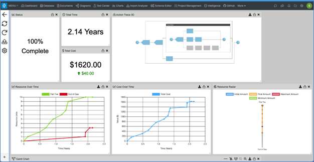
Figure 10. A Single Discrete Event Simulation Run.

To see the impact of many executions we use the Monte Carlo simulator. The results of this simulation for 1000 runs are shown in Figure 11.

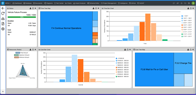
Figure 11. Monte Carlo Calculations for 1000 Iterations.

As a result, you can see that for about a year in operation, the owner of this vehicle can expect to spend an average of over $3,956. However, you could spend as much as $9,000 over two years.

For more detailed analysis, you can click the download button in each window for reports that detail these runs (see Figure 12).

Figure 12. A Variety of Reports Are Available from Each Window.

This problem serves as a starting point, but the potential for analysis using this method extends far beyond simple scenarios. Incorporating failure modes into your model as you create it is crucial. Model-Based Systems Engineering is an incredibly effective tool for FMECA, allowing for in-depth analysis and enhanced understanding of potential failures.